Monte Carol Tree

Monte Carlo tree search (MCTS) is a widely used heuristic search algorithm for gaming AI. For a game involving two opponents, the decision-making is modeled as a tree, and the problem of winning the game is formalized as traversing, expanding, and simulating the tree. Before MCTS, deterministic algorithms like Alpha-Beta tree search were used, which enumerates all potential states to find the optimal next move. However, these approaches are not feasible for those games that have large action space, as the tree grows exponentially for every next move. Monte Carlo tree search, as a probabilistic algorithm, solves this problem. The basic idea is rather than exploring every new move, we select the promising moves and focus on them. In this way, we shrink the tree size and save time by ignoring those unpromising moves. The algorithm is probabilistic because we use the Monte Carlo approach to determine which moves are promising.

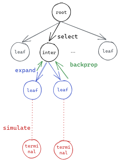
MCTS is essentially a tree search algorithm with certain policies and constraints. The algorithm involves four operations:

• Expansion: When visiting a tree node, if the node has not been visited before, it will be a leaf node. If so, we expand this node, i.e. creating a child node for each potential move from the state that this node represents.
• Selection: For a given tree node, if the node has been visited before, it will not be a leaf node, so we traverse the tree further by selecting the most promising child node with some evaluation function. In multi-arm bandit problems, it is typical to use Upper Confidence bound applied to Trees (UCT) as an evaluation function.
• Simulation: For each leaf node derived from expansion, we run simulations of this node by randomly applying moves until it reaches a terminal state, i.e. win, draw or lose. The simulation should run in large quantities to provide a good estimate. This is where “Monte Carlo” comes from.
• Backpropogation: Based on each simulation of a leaf node, the simulation results (number of wins, draws and loses) are backpropagated to the ancestors so we can get a more accurate estimate of the best next move.

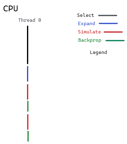
Our baseline is a CPU-powered, single threaded MCTS algorithm.

Or in pesudocode:

run(){
    for(i in range(MAX_EXPAND_STEPS)){
        traverse(root);
    }
}

traverse(Node node){
    if(!isLeaf(node)){
        // if it is not a leaf node, traverse further down the tree
       if(!isTerminal(node)) traverse(select(node));
    }else{
        expand(node);
        for(child:node->children){
            for(i in range(SIM_TIMES)){
                backprop(simulate(node));
            }
        }
    }
}

Node select(Node node){
    // select one of the children of the node with greatest UCB
}

expand(Node node){
    // apply game logic to expand the tree
}

Result simulate(Node node){
    // random simulate to the terminal state
}

backprop(Result){
    // backprop the result of node simulation to its ancestors
}

Game of Reversi

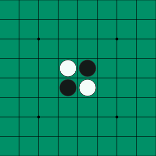
We choose Reversi (or “othello” as my partner calls it) as the game to test and parallelize our MCTS on. Reversi is a game involving two players playing either white or black stones on an N\times N board. The board is initialized with the four blocks in the center filled with 2 white and 2 black stones. The white side moves first and then two players move in turns. On every move, the player can only place the stone in a block so that there exists another stone with the same color in a vertical/horizontal/diagonal line with the new stone, and there are contiguous stones between them with the opposite color. After such a move is made, all the opposite color stones between the newly placed stone and the other existing stone flip their color (i.e. change to the same color as the newly placed stone). When a player cannot make such a move, the game terminates, and the player with more stones of his color on the board wins the game.

The status of all the blocks on the board is considered as a state. And such a state is corresponding to a node in the MCTS tree as shown in the overview figure. Every time our algorithm needs to choose its next action, it starts with the current board status as the root node. The four operations of the MCTS are executed as follow:

• Expansion: Searches for all possible actions it can make based on the current status. Expand them as new leaf nodes.
• Selection: Among all the nodes (i.e. board status after taking those actions), chooses the one that holds the highest UCB value.
• Simulation: Based on the chosen node (board status), keeps randomly choosing the next action it or its opponent can make until the game terminates.
• Backpropagation: Update all the ancestors with the number of wins, draws and loses in simulations.

Approach

Parallel Simulation

We first did a profiling on the baseline with gprof. The result is attached below:

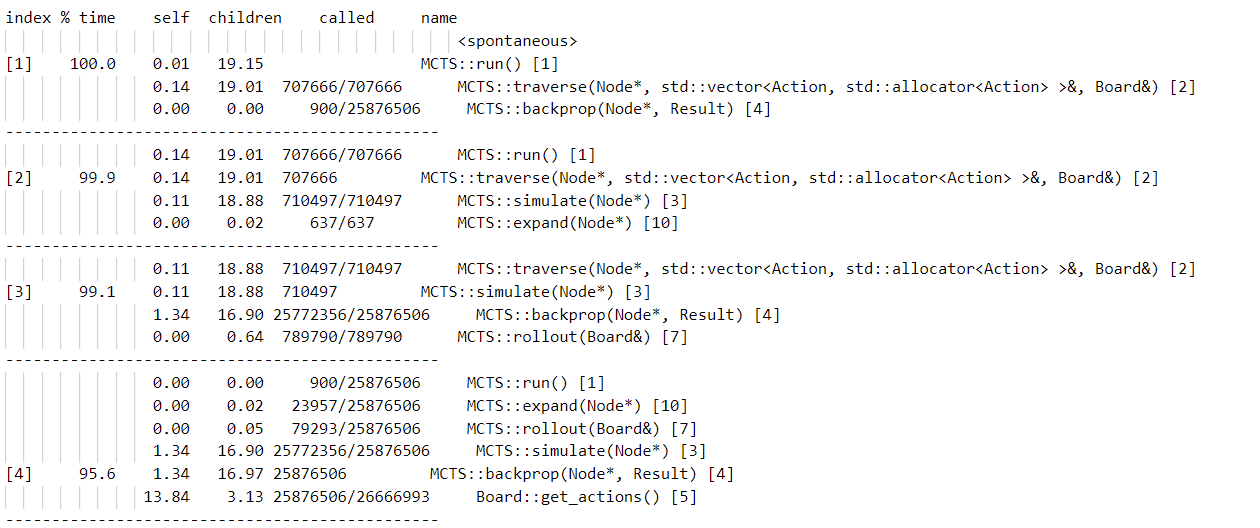
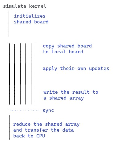
Based on the output of profiling of the baseline, we determine that the most intuitive and effective way of parallelizing this algorithm is to parallel the simulation and backpropagation process. Since each process is independent, we can safely run them simultaneously. To achieve that, we just need to implement a simulation kernel in CUDA. Notice that we also benefit from the fewer calls to backprop because we are able to reduce the simulation results from the simulation kernel to a single BackPropObj and backpropagate that object along the tree.

Since the GPU has less computation power in sequential code than CPU, we must carefully implement the kernel to achieve the maximum performance and avert the overhead.

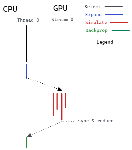
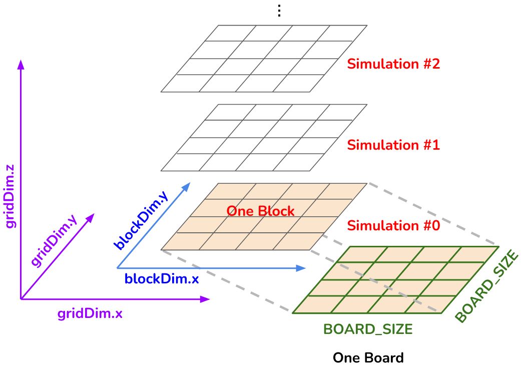
Below is the arrangement of GPU threads. Every block runs one simulation, where every thread is responsible for exactly one location on the board. The Z dimension of the grid is exploited to run multiple simulations in parallel.

As we seek more parallelization, there are mainly two directions:

• We seek a higher level of parallelism in hardware, e.g. the multi-threading of CPU and multi-streaming of GPU.
• We perform workload partition so that we can explore the computation power of the CPU and GPU at the same time. This is what is called heterogenous computing

Completely Parallel MCTS

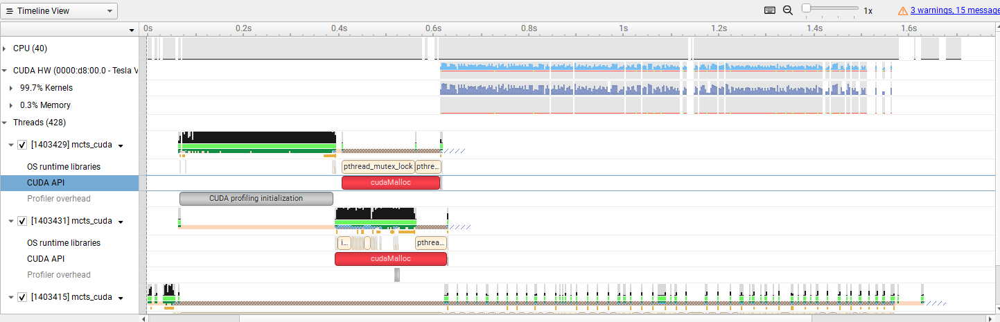
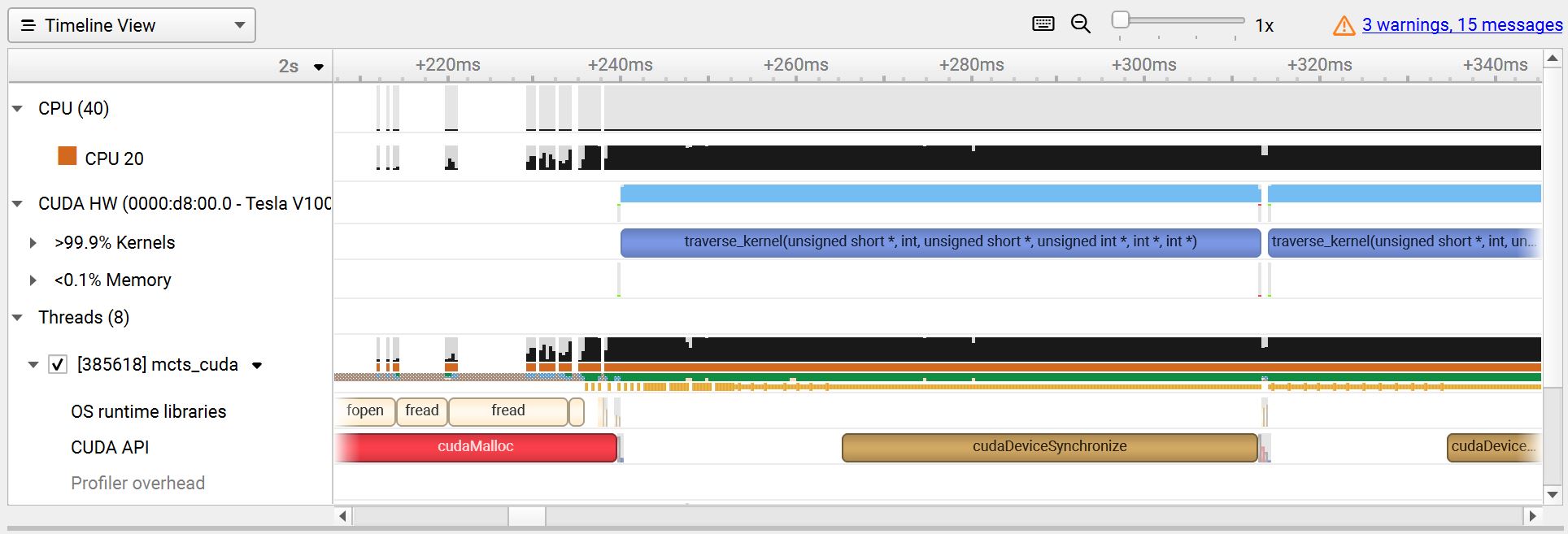
The timeline graph of the parallel simulation described in the previous section is as follows. We can see a large overhead of cudaMemAlloc(large chunk of red rectangle) and some cudaMemCpy (smaller chunks of red rectangles) that causes the program to synchronize.

We found the considerable overhead of cudaMalloc and the cost of synchronization between the host and device introduced by cudaMemcpy. We tried to optimize that by making the kernel call asynchronous using threads. This prevents one iteration of traverse from blocking another iteration of traverse. Leveraging parallelism to this level does not follow the rule of MCTS strictly because dependency exists for a serial MCTS. The selection result of the following iteration depends on the simulation result of the previous iteration. If we do it in parallel, we can not make sure that all iterations can select the “most” promising node so far to simulate. However, since MCTS is a heuristic and probabilistic algorithm, we argue that this deviation of can be compensated by the huge amount of simulations we gain by parallelization.

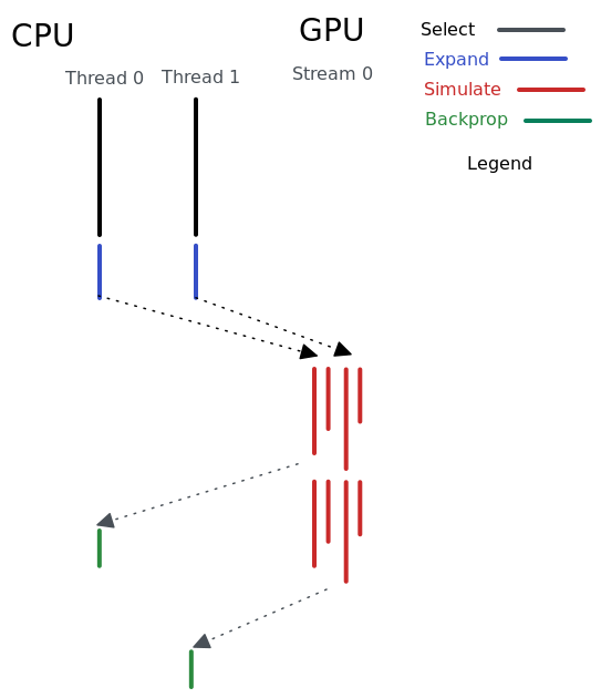
Our first trial is simply to wrap the call to the kernel with a thread object and join all threads in the end. However, this approach didn’t work well. By analyzing the performance profile, we found that the only benefit we gain is paralleled cudaMalloc (the red rectangles in the figure). The kernel code still ran in serial, and the performance gain with respect to the naive parallelized simulation is negligible.

The reason behind this is that the multi-thread strategy can only parallelize the work that is done on the CPU. Once the kernels are launched, they are all assigned to Stream 0 on the GPU by default, and all work on the same stream of a GPU is executed in serial.

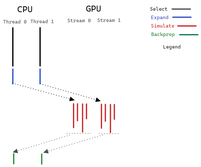
To make it more parallel we exploit the power of CUDA streaming. CUDA streaming is the ability to perform multiple CUDA operations (data transfer, kernel computation, etc.) In our case, it means we can do cudaMemcpyAsync and simulation kernel completely in parallel in different streams. With that, we can say our program is “completely parallelized”.

Heterogenously Parallel MCTS

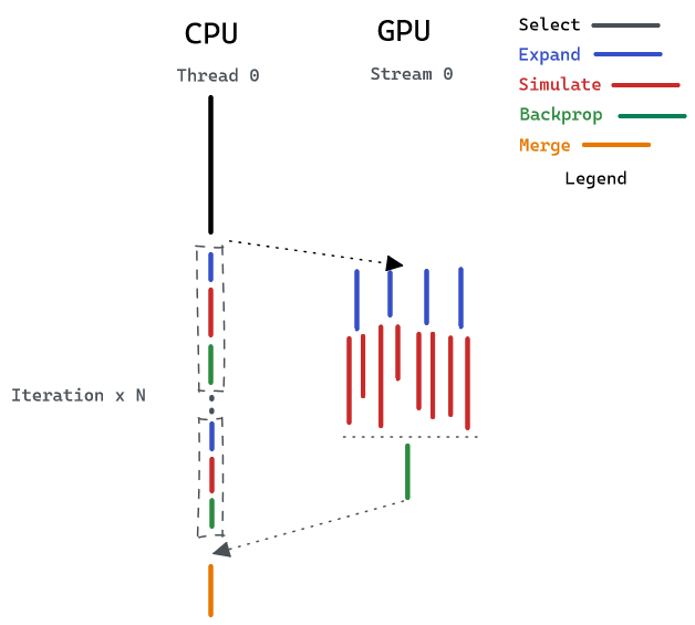
In our Completely Parallel MCTS algorithm, we achieve very high parallelism in the simulation section on the GPU. Also, the CPU is able to parallelize the expand section by taking advantage of multiple threads. However, one issue with this strategy is that the parallelism is limited by the number of CPU cores and the number of GPU streams. If we want to have more expansions and simulations (i.e. larger maximum expansion times and maximum simulation times), the strategy would eventually reach a speedup limit. Therefore, we also explore the parallelism between CPU and GPU. We divide the workload into two parts - one for the CPU, one for the GPU. On the GPU side, we develop a new kernel that can do all the expansion, simulation, and backpropagation parts. This kernel utilizes more hardware resources in the GPU to achieve greater parallelism. At the same time, we let the CPU handle the other part of the work. Because the CPU has a shorter execution latency on a single iteration than the GPU, it can run multiple iterations before the GPU finishes and finally merge the results.

As you can see from the above figure, the results can only be merged after both CPU and GPU complete computing. That means the total latency of the program is determined by the slower core. Therefore, we must balance the workload distribution so that CPU and GPU will take approximately the same amount of time to finish.

The first figure below shows the case when the GPU is assigned more workload and takes longer to compute. The CPU becomes idle after finishing its own work while the GPU is still running the kernel. In such a situation, the workload is unbalanced and the total latency is determined by the GPU kernel. The second figure shows the case when both CPU and GPU finish computing at almost the same time.

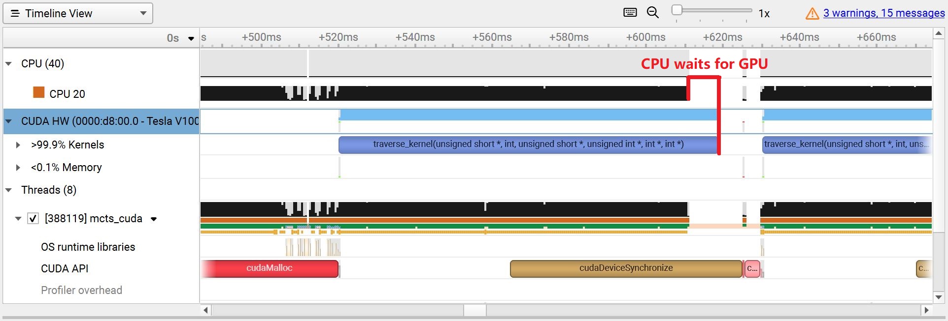CPU waits for GPU

Balanced workload

Results

The run time of the different parallel MCTS algorithms was collected by measuring the average time for the algorithms to make one action over 20 different action makings. All time was measured in milliseconds (ms). Here is the compiled table of all the timing results we get from the approaches we implemented. The parameters we scaled upon is the number of expansion and the number of simulations we perform for each expansion. We tested the scaling of both factors for each choice of parameter (#simulation = #expansion = parameter) to examine the capability of the program regarding the scaling of both exploitation and exploration.

#sim/expand	Baseline	Parallel Simulation	Completely Parallel	Heterogenous
10	378.97	44.36	41.21	506.27
20	1146.55	80.36	74.91	657.31
50	4563.89	154.25	130.31	2422.40
100	6886.91	200.83	226.46	/

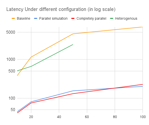
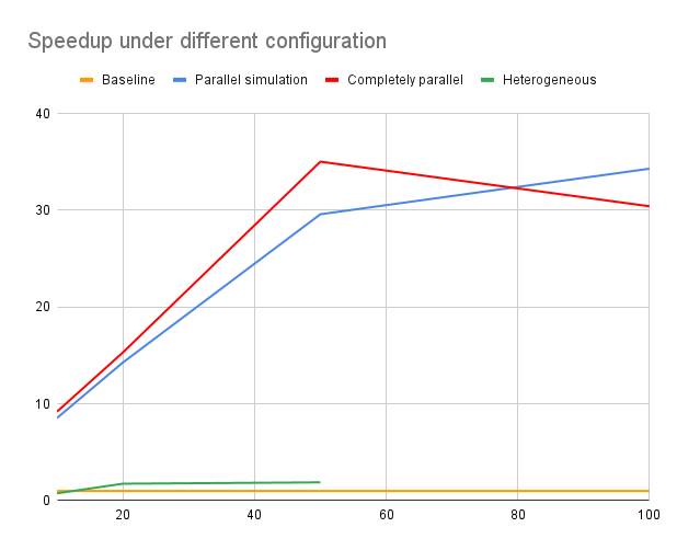
We didn’t measure the heterogenous approach with simulation and expansion times 100 because it costs more than 5 minutes to finish the whole program. A visualization of the above statistic is provided.

Conclusion

All of our approaches are significantly better than the baseline model. We gained two insights from the results:

• The highest level of parallelization might not work best due to hardware constraints.
• Heterogenous computation needs careful workload balancing to boost performance.

Level of Parallelization

Normally we think the more paralleled the algorithm is, the better performance it will gain. This is not necessarily the case with our experiment. First of all, there’s overhead for parallel setup (memory allocation and copy, CUDA stream instantiation, context switch, etc). Besides that, GPU does not execute serial code as efficiently as the CPU, which means loading more serial code on GPU degrades the performance.

The first approach (i.e. parallelized simulation) is probably the best taking code complexity and performance gain into consideration. This further reminds us of the best practice in designing CUDA programs: optimize memory access pattern, decrease kernel complexity and avoid transcendental functions.

The second approach (i.e. completely parallelized) should theoretically be faster than the first one but the result shows it is no better. On further inspection, we found that streams in CUDA programming is a best-effort parallel feature, which means it is only applicable when there are available GPU resources to fit a kernel. Therefore, it is “better to use stream when you have several small and different kernels that does not depend on each other.” In our case, the kernel we launch does not depend on each other, but they have similar memory access pattern which means they are prone to blocking each other. Therefore, they are not executed in fully parallel. The timeline figure below shows that although they are in different streams, the kernels are still executed in serial. That’s why the benefit we obtain is negligible.

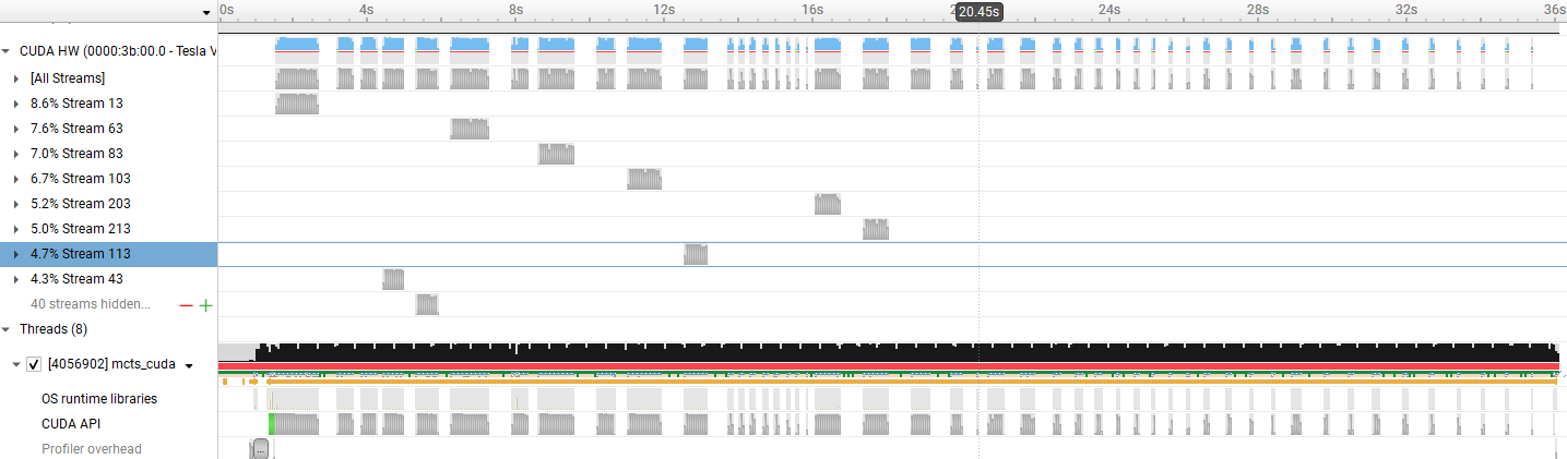Closer inspection on the completely parallel MCTS

Heterogenous Computing

In a normal usage scenario, the CPU is used as a manager and the GPU as a worker. In the third approach, we explored the possibility of using the computing power of the CPU and GPU simultaneously and finding a sweet point where they are able to finish the computation at the same time.

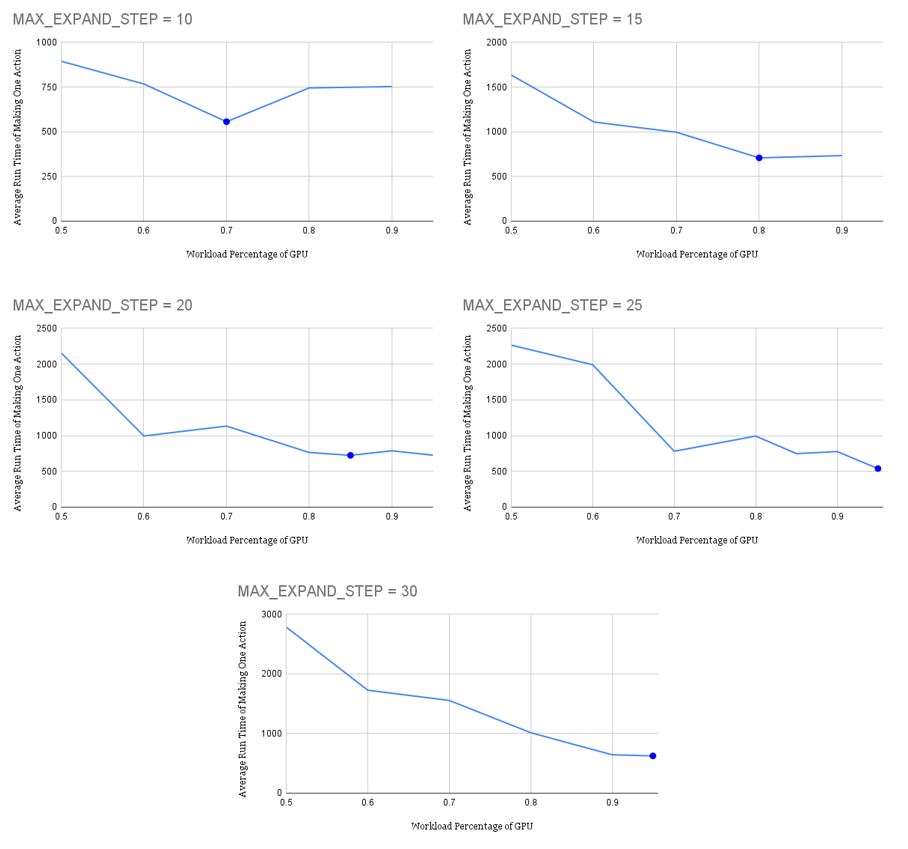
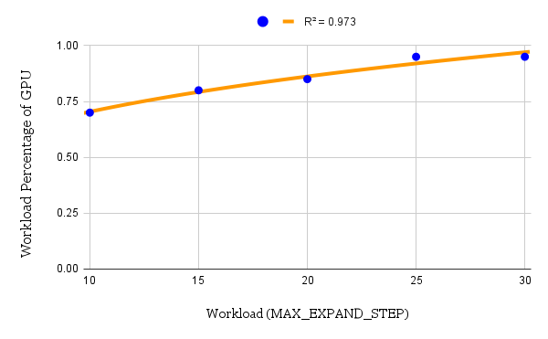
Multiple tests have been run with different workloads and workload distributions. Specifically, the workload is determined by MAX_EXPAND_STEP, which represents the number of iterations of the expand-simulate-backpropagate group. The results are shown in the first figure below. The blue spot in every graph represents the best workload percentage assigned to the GPU that results in the shortest run time. And the relationship between this percentage and the total workload is shown in second figure. As the total amount of workload increases, the best percentage that gives the shortest run time also increases.

We try to fit the data points into a trending curve and find that the exponential equation

\text{GPU load} = 0.36\times \texttt{MAX\_EXPAND\_STEP}^{0.292}

gives the highest R-square value when 10 \leq\texttt{MAX\_EXPAND\_STEP} \leq 30. When MAX_EXPAND_STEP grows beyond 30, the percentage will converge to 1.0. The percentage trends in this way because GPU exploits higher parallelism than CPU. As the workload assigned to CPU and GPU increases, the run time of CPU increases in an almost linear manner, while the run time of GPU barely increases. Therefore, only by assigning more work to the GPU can the run time of both CPU and GPU keep the same as the workload increases.

Epilogue

We call it a failure since the two approaches we proposed did not work well and the good old one wins. But